In theoretical photochemistry, we simulate what happens when molecules and materials absorb light. In order to excite electrons in organic materials, a requirement for photovoltaic devices, the light has to be in the ultraviolet range of the electromagnetic spectrum. To characterise molecules, a UV/Vis spectrometer measures how absorption varies with the energy of the incident light. We can simulate this process using calculations, and plot a spectrum, without ever going into the lab.

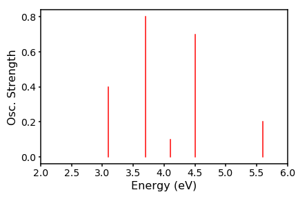
In this post I will discuss the simplest method to simulate a spectrum, using a hypothetical set of absorption energies for a single molecular conformation. The x-axis will be a set of electronic excitation energies, and the y axis is the associated oscillator strength. The oscillator strength, simply put, is a measure of the likelihood, or favourability, that at a specific energy of light, the energy will be absorbed by the molecule.

energies=[3.1, 3.7, 4.1, 4.5, 5.6]
osc=[0.4, 0.8, 0.1, 0.7, 0.2]

We can plot a line spectrum using:

fig,ax=plt.subplots(figsize=(6,4))
for energy,osc_strength in zip(energies,osc):
    ax.plot((energy,energy),(0,osc_strength),c="r")
ax.set_xlabel("Energy (eV)",fontsize=16)
ax.xaxis.set_tick_params(labelsize=14,width=1.5)
ax.yaxis.set_tick_params(labelsize=14,width=1.5)
for axis in ['top','bottom','left','right']:
    ax.spines[axis].set_linewidth(1.5)
ax.set_xlim(2,6)
ax.set_ylabel("Osc. Strength",fontsize=16)
plt.tight_layout()

to produce:

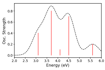
Thats all well and good, but does not represent what really happens in a spectrometer, since there are huge numbers of molecular conformations, which will all have slightly different oscillator strengths. Therefore, we have a distribution about our vertical line. We can crudely approximate this distribution to be gaussian and interpolate between the energies to generate a peaks. To achieve this we need to code up the gaussian distribution. To get our set of y-values, we run across an array of M energies (our x-values) and use as our reference each of our N excitation energies E, which sit at the centre of the distribution. The scaling factor is the associated oscillator strength f. Our resulting spectrum will thus take the form:

We can define a function that computes the above equation as:

def spectrum(E,osc,sigma,x):
    gE=[]
    for Ei in x:
        tot=0
        for Ej,os in zip(E,osc):
            tot+=os*np.exp(-((((Ej-Ei)/sigma)**2)))
        gE.append(tot)
    return gE

We can call this function using our fictitious energies and oscillator strengths, choosing sigma as 0.4 eV and x to run over 500 points within an 6 eV window:

x=np.linspace(0,6, num=500, endpoint=True)
simga=0.4
gE=spectrum(energies,osc,sigma,x)

We can then plot x against gE to have a nice broadened spectrum:

fig,ax=plt.subplots(figsize=(6,4))
ax.plot(x,gE,"--k")
for energy,osc_strength in zip(energies,osc):
    ax.plot((energy,energy),(0,osc_strength),c="r")
ax.set_xlabel("Energy (eV)",fontsize=16)
ax.xaxis.set_tick_params(labelsize=14,width=1.5)
ax.yaxis.set_tick_params(labelsize=14,width=1.5)
for axis in ['top','bottom','left','right']:
    ax.spines[axis].set_linewidth(1.5)
ax.set_xlim(2,6)
ax.set_ylabel("Osc. Strength",fontsize=16)
plt.tight_layout()

We can even play around with our line widths by changing the standard deviation:

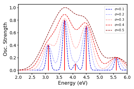
On my github, I have a python program that does all of this automatically, and even converts the y-axis to a more chemically relevant unit (L/mol/cm). It takes as input Gaussian 09 TD-DFT output files, parses it for the energies and oscillator strenghts, and will automatically render an absorption spectrum. It can do this for multiple input files at the same time so that you can overlay spectra - feel free to use it in your work!

md

Back to posts